Molecular Graphs
MolScope supports two common graph views for molecular ML:
- Chemical graphs: atoms are nodes, covalent bonds are edges.
- Spatial contact graphs: atoms, residues, or coarse-grained beads are nodes; edges mean two units are close in 3D space.
Use chemical graphs when local chemistry and bond topology matter: small-molecule property prediction, functional groups, valence-sensitive tasks, or atomistic message passing. Use contact graphs when folded shape and neighborhood structure matter: protein residue networks, interfaces, binding-site context, NMR conformer comparison, or coarse-grained models.
Atom and bond graphs
The dependency-free atom graph layer treats atoms as nodes and explicit or inferred bonds as edges:
g = mol.to_graph()
g.n_atoms, g.n_bonds
g.node_features()
g.node_features("ml")
g.edge_features("ml")
g.feature_matrices(return_names=True)
g.edge_types  # bond orders, 1.0 when inferred or unknown
g.formal_charges
Node attributes include element, atomic number, mass, coordinates, and, when the
source file has them, atom name, residue name/id, chain and formal charge. Edge
attributes include endpoint indices, interatomic distance and bond order
(1.0 for inferred or unknown orders).
Feature presets keep ML columns stable:
- Node
default: atomic number and mass. - Node
basic: atomic number, mass, formal charge. - Node
ml: fixed element one-hot features, atomic number, mass, formal charge, aromatic flag. - Edge
default: distance. - Edge
basic: distance and bond order. - Edge
ml: distance, bond order, aromatic flag.
ms.list_presets("graph") (or molscope presets graph --features) prints these,
the residue-graph presets, and the exact feature names each one expands to.
Use optional RDKit-backed aromaticity when building the graph:
g = mol.to_graph(include_chemical_features=True)
Configurable edges for 3D GNNs
By default edges are covalent bonds (explicit or geometrically inferred). For
3D GNN architectures it is standard to build the edge set from spatial proximity
instead, which to_graph supports directly:
g = mol.to_graph(knn=12)                   # k-nearest-neighbour edges
g = mol.to_graph(radius=8.0)               # all atom pairs within 8 Å
g = mol.to_graph(delaunay=True)            # Delaunay / Voronoi adjacency
g = mol.to_graph(knn=12, min_seq_sep=3)    # k-NN, minus trivial local contacts
g = mol.to_graph(min_seq_sep=3)            # filter covalent/inferred bonds too
knn=k connects each atom to its k nearest neighbours by Euclidean distance.
The per-node neighbour lists are symmetrised by union, so an edge survives when
either endpoint ranks the other among its k nearest. k is capped at n - 1.
radius=r connects every atom pair within r angstrom, reusing the same fast
KD-tree / cell-list search as Molecule.contacts.
delaunay=True builds edges from the 3D Delaunay triangulation — equivalently,
Voronoi adjacency — a threshold-free, density-adaptive graph that avoids the
dense-core/exposed-loop disparities of a fixed cutoff. It requires SciPy (the
[fast] extra); unlike knn/radius there is no pure-NumPy fallback. Note that
a raw Delaunay graph introduces some long edges across surface concavities and
the convex hull, so pair it with min_seq_sep (or filter by edge_distances)
when those matter.
At most one of knn, radius, delaunay and an explicit bonds= array may be
given.
min_seq_sep drops same-chain edges whose residue-id separation
|resid_i - resid_j| is below the threshold — the standard way to remove
trivial local backbone interactions (min_seq_sep=3 keeps only contacts at
least three residues apart in sequence). Edges that bridge two chains are always
kept, and the filter needs residue ids; it applies to every edge mode. These
options pass straight through the exporters, e.g.
mol.to_pyg_data(radius=8.0, min_seq_sep=3, node_preset="ml").
Residue contact graphs
Residue contact graphs use residues as nodes and spatial contacts as edges:
rg = mol.to_residue_contact_graph(cutoff=8.0, method="ca", min_seq_sep=4)
rg.n_residues, rg.n_contacts
rg.node_features("ml")
rg.edge_features("ml")
The contact construction method controls the edge meaning:
method="ca": alpha-carbon distance, with centroid fallback when CA is absent.method="com": residue centre-of-mass distance.method="min": closest inter-residue atom distance.
min_seq_sep removes local same-chain contacts such as adjacent residues, which
is useful when you want long-range tertiary contacts instead of backbone
neighbors. chain_mode="intra" keeps only within-chain edges, while
chain_mode="inter" keeps only between-chain edges.
Residue node features include residue-type one-hot columns and residue atom count. Contact edge features include distance and the contact method:
x, edge_attr, node_names, edge_names = rg.feature_matrices(return_names=True)
Coarse interaction labels
Pass annotate_interactions=True to label each contact edge with one coarse
interaction class, computed from residue chemistry and atom-level geometry:
rg = mol.to_residue_contact_graph(annotate_interactions=True)
rg.edge_interactions          # one label per edge
rg.interaction_one_hot()      # (E, 7) categorical edge feature for ML
G = rg.to_networkx()          # each edge carries an `interaction` attribute
The labels are mutually exclusive, assigned by precedence (most specific first):
disulfide (CYS SG–SG < 2.5 Å) > ligand (a non-standard, non-water residue) >
salt_bridge (basic↔acidic charged side-chain atoms < 4 Å) > covalent
(sequence-adjacent same-chain neighbours) > hydrophobic (both hydrophobic, side
chains in contact) > polar (both polar/charged, side chains in contact) >
proximity (everything else, including water contacts). The vocabulary is
molscope.RESIDUE_INTERACTION_LABELS.
These are geometric/contact heuristics, not binding-energy terms, and they need per-atom names to resolve the chemistry (degrading to covalent/ligand/proximity otherwise).
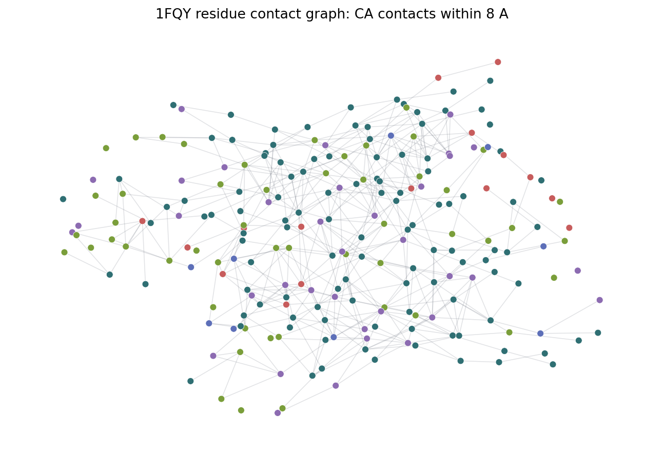
The image above is generated by examples/residue_contact_graph.py. It projects
residue representative coordinates to a 2D plane, colors residues by broad
residue class, and draws non-local CA contacts within 8 A.
Export
NetworkX export:
G = mol.to_networkx()
RG = rg.to_networkx()
PyTorch Geometric export:
data = mol.to_pyg_data()
data = mol.to_pyg_data(node_preset="ml", edge_preset="ml")
residue_data = rg.to_pyg_data(node_preset="ml", edge_preset="ml")
DGL export:
dglg = mol.to_dgl_graph()
dglg = mol.to_dgl_graph(node_preset="ml", edge_preset="ml")
residue_dgl = rg.to_dgl_graph(node_preset="ml", edge_preset="ml")
Edge attributes for 3D GNNs
Both exporters attach an is_covalent edge flag (PyG data.is_covalent, DGL
edata["is_covalent"], NetworkX edge covalent). It is all-True for a
bond-derived graph, but for a spatial graph (knn/radius/delaunay) it marks
which contacts coincide with real covalent bonds, so a model can tell chemical
bonds from proximity contacts.
For SchNet/EGNN-style models, pass include_displacement=True to add a directed
relative-displacement vector edge_vec = pos[dst] - pos[src] per edge
(antisymmetric: the reverse edge holds its negation):
g = mol.to_graph(radius=6.0)
data = g.to_pyg_data(include_displacement=True)   # data.edge_vec, data.is_covalent
dglg = g.to_dgl_graph(include_displacement=True)   # edata["edge_vec"], edata["is_covalent"]
pos and edge_index are exported regardless, so equivariant models can also
derive r_ij themselves; include_displacement is a convenience that
precomputes it.
Install the exporter backend you need:
pip install "molscope[graph]"  # NetworkX
pip install "molscope[pyg]"    # PyTorch Geometric
pip install "molscope[dgl]"    # DGL
pip install "molscope[gnn]"    # all graph backends
For custom CUDA, ROCm, Apple Silicon, or cluster builds, install the matching PyTorch stack from the backend project's instructions first.
Building a dataset in one call
To go from a folder of structures to a split, label-joined set of graphs without
writing the loop yourself, use build_dataset:
import molscope as ms

ds = ms.build_dataset(
    "data/*.pdb",                 # glob, list of paths, or list of Molecules
    fmt="pyg",                    # "pyg" | "dgl" | "networkx" | "raw"
    node_features="ml",
    edge_features="geom",
    pe="laplacian", pe_k=8,       # optional positional encodings (pyg/dgl)
    labels="labels.csv",          # optional id->target table, joined by file stem
    split=(0.8, 0.1, 0.1),        # optional random train/val/test split
    n_jobs=4,
)

print(ds.summary())
ds.train, ds.val, ds.test         # framework graph objects, the split as lists
ds.save("out/")                   # graphs + a manifest.json
It is a thin wrapper over the exporters above, so fmt="pyg"/"dgl" need their
extras while fmt="raw" (a MolecularGraph) and fmt="networkx" run on the
core install. Unreadable inputs are skipped and recorded in ds.skipped unless
you pass on_error="raise".
Cache featurisation across runs
Featurising a large corpus is the slow part. Pass cache_dir= to store each
structure's graph on disk so later runs reuse it instead of recomputing:
ds = ms.build_dataset("data/*.pdb", fmt="pyg", cache_dir=".graph_cache")
# tweak labels or the split and rebuild — only new/changed files re-featurise
ds = ms.build_dataset("data/*.pdb", fmt="pyg", cache_dir=".graph_cache",
                      labels="labels.csv", split=(0.8, 0.1, 0.1))
Each cache entry is keyed by the file's content plus the featurisation
options (fmt, the feature presets, pe, self_loops, ...), so editing a
structure or changing an option re-featurises just that input automatically.
labels and split are applied after loading and are not part of the key, so
re-labelling or re-splitting a cached set is free. In-memory Molecule sources
are not cached (they have no stable on-disk identity), and a corrupt entry is
simply recomputed.
Build from RCSB accessions (benchmark tables)
Published benchmarks usually arrive as a table of PDB accessions and a target
column. fetch_dataset is the adapter for that shape: it
downloads each accession from the RCSB (cached under root, so a rerun does not
re-download), then runs build_dataset on the files.
labels = {"1fqy": 0.0, "3ptb": 1.0, "1ubq": 0.0}    # your accession -> target
ds = ms.fetch_dataset(
    labels.keys(),
    labels=labels,                # or a CSV path keyed by the lowercased id
    fmt="pyg",
    node_features="ml",
    split=(0.8, 0.1, 0.1),
    cache_dir=".graph_cache",     # forwarded to build_dataset's featurisation cache
)
Accessions are case-insensitive. A download that fails (network error, unknown
id) is recorded in ds.skipped and skipped rather than aborting the build,
unless you pass on_error="raise". MolScope does not ship curated label tables —
bring your own from the benchmark you are reproducing.
Mini-batches for a training loop
For fmt="pyg" or fmt="dgl", ds.loader() hands back
the framework's batching DataLoader so you can drop straight into a training
loop:
train_loader = ds.loader("train", batch_size=32)   # shuffles by default
val_loader   = ds.loader("val", batch_size=64)      # no shuffle

for batch in train_loader:
    out = model(batch)            # a batched PyG Data / DGL graph
    ...
Pass split=None (the default) to loop over the whole dataset, or "train" /
"val" / "test" for a subset built with split=. The train split shuffles
each epoch and the others do not, unless you set shuffle= explicitly; extra
keywords (num_workers, drop_last, ...) are forwarded to the underlying
loader. That is where MolScope stops: it gives you DataLoader-ready batches, but
no training loop or model code.
Standardise regression targets without leaking
For fmt="pyg" regression, ds.standardize_targets() fits the target mean and
standard deviation on the train split only, rewrites every graph's data.y
into standardised space, and returns a TargetScaler:
scaler = ds.standardize_targets()        # fit on train, applied to all data.y
...
pred_angstroms = scaler.inverse_transform(model(batch))  # back to physical units
Fitting on train alone keeps validation and test out of the statistics — the
normalisation mistake that quietly inflates scores. ds.labels keeps the
original values.