Coarse-Graining¶

Coarse-graining maps an atomistic structure onto a smaller set of beads. In MolScope this is deliberately educational: it helps you inspect mappings, compare representations, and build graph prototypes. It does not generate validated production simulation topologies.

cg = mol.coarse_grain("residue_com")
cg = mol.coarse_grain("residue_centroid")
cg = mol.coarse_grain("martini")

The result is still a Molecule, so it can be plotted, transformed, converted to a graph, and analyzed.

Built-in teaching mappings¶

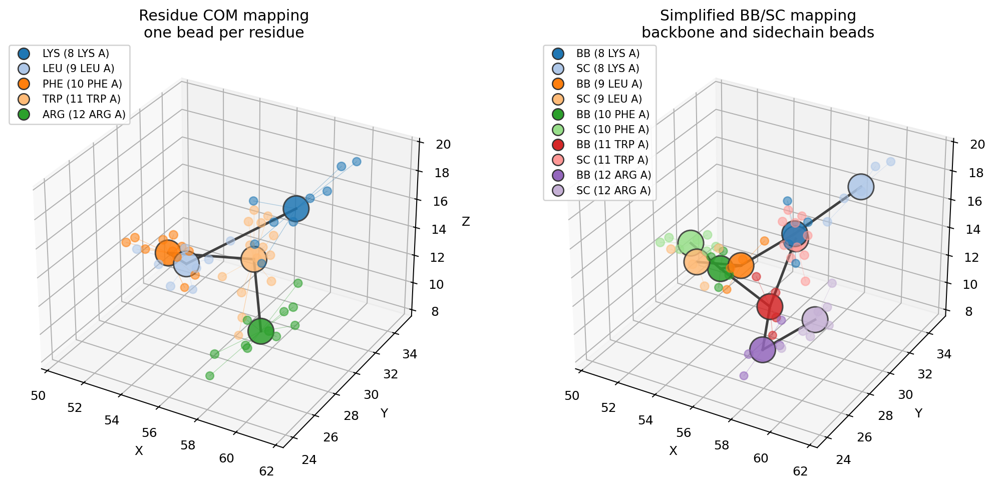
Residue centre of mass¶

"residue_com" collapses each residue to one bead at the mass-weighted centre of all atoms in that residue:

mol = ms.read("examples/data/1fqy.pdb")
cg = mol.coarse_grain("residue_com")

len(mol), len(cg)        # 1661 atoms -> 226 residue beads
cg.atom_names[:5]        # residue names carried as bead names

Mass weighting matters: a centre of mass is pulled toward heavier atoms, while a centroid is the unweighted average of coordinates. Use "residue_centroid" when you want the geometric centre instead:

com = mol.coarse_grain("residue_com")
centroid = mol.coarse_grain("residue_centroid")

Backbone/sidechain beads¶

"martini" is a simplified backbone/sidechain split inspired by Martini-style coarse-graining:

bb_sc = mol.coarse_grain("martini")
bb_sc.atom_names[:6]     # ['BB', 'SC', 'BB', 'SC', ...]

For each residue, backbone atoms (N, CA, C, O, OXT) become a BB bead and non-hydrogen sidechain atoms become an SC bead when present. MolScope then adds a simple bead graph: within-residue BB-SC bonds plus sequential BB-BB links along each chain.

Virtual sites can be added explicitly when you want a coordinate derived from existing beads without treating it as another atom-assignment bead:

bb_sc = mol.coarse_grain(
    "martini",
    virtual_sites=[{"name": "MID", "parents": [0, 2]}],
)

The virtual site is appended to the CG coordinates, marked with cg.virtual_sites, preserved in mapping JSON, drawn as a distinct marker, and exposed as a virtual_site flag in graph exports. Parent references are bead indices in the CG model before virtual sites are appended; names are accepted only when they are unique.

This is the useful concept to learn from Martini: represent groups of atoms as interaction sites, preserve an interpretable molecular shape, and work at lower resolution. Real Martini models also require bead types, bonded terms, nonbonded parameters, charges, exclusions, virtual-site topology sections, validation against reference atomistic/experimental behavior, and toolchain-specific topology files. MolScope does not attempt those production steps.

Custom residue mappings¶

mapping = {"ALA": {"BB": ["N", "CA", "C", "O"], "SC": ["CB"]}}
cg = mol.coarse_grain(mapping)

Custom index mappings¶

cg = mol.coarse_grain(
    {"head": [0, 1, 2, 3], "tail": [4, 5, 6, 7]},
    bonds=[("head", "tail")],
)

Name-based bonds are intended for unique bead names. Repeated names such as BB and SC are ambiguous across residues; use bead indices for those.

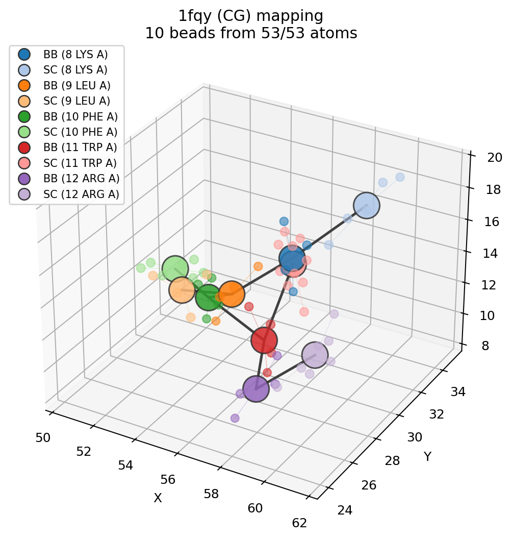
Visualise the mapping¶

plot_mapping shows how the beads sit on top of the atoms they replace. Each atom is coloured by the bead it was folded into, every bead is drawn as a large translucent sphere at its position, thin lines join atoms to their bead, and the CG bond network is drawn between beads. Atoms left unassigned appear as faint grey crosses.

import molscope as ms

fragment = ms.read("examples/data/1fqy.pdb").select(resid=(8, 12))
cg = fragment.coarse_grain("martini")

ms.plot_mapping(fragment, cg)     # or: cg.plot_mapping(fragment)

Martini bead mapping of an Aquaporin-1 fragment, atoms coloured by bead

For an interactive, rotatable overlay in a Jupyter notebook, use view_mapping (needs the [viz] py3Dmol extra). It renders the atomistic structure as a semi-transparent model with the beads drawn as solid spheres on top, so students can rotate the mapping and see exactly which atoms each bead replaces:

cg.view_mapping(fragment)                       # or: ms.view_mapping(fragment, cg)
cg.view_mapping(fragment, atom_style="cartoon") # cartoon backbone for proteins

To compare mapping resolutions side by side, run:

uv run python examples/coarse_graining.py

Residue COM and simplified BB/SC mappings for the same Aquaporin-1 fragment

Pass the structure the CG model was built from (same atom order). The atom-to-bead lines are drawn automatically for small structures; toggle them with show_assignment=True/False, and the bead legend appears when there are few enough beads to stay readable (max_legend).

From the command line¶

molscope coarse-grain maps a structure to beads and writes a coordinate file you can open in PyMOL, ChimeraX, or Mol*:

molscope coarse-grain structure.pdb --mapping martini --out cg.pdb
molscope coarse-grain --fetch 1fqy --mapping residue_com --out cg.pdb
molscope coarse-grain structure.pdb --mapping martini        # summary only, no file

--mapping is residue_com (default), residue_centroid, or martini. The output format follows the --out extension (.pdb, .cif, or .xyz); beads are written as pseudo-atoms with their bead names (BB/SC for Martini), and the bead bond network is written as CONECT records for .pdb output. .cif and .xyz carry coordinates only, so prefer .pdb when you want the network to show up in a viewer. The command always prints the mapping coverage.

Inspect the bead assignment¶

Every coarse-grained Molecule carries a structured report describing exactly which atoms went into each bead:

cg = mol.coarse_grain("martini")
report = cg.coarse_grain_report

print(report.coverage())          # "426 beads from 1661/1661 atoms"
print(report.n_beads, report.n_assigned, report.n_dropped)

first = report.beads[0]
print(first.name, first.resname, first.resid, first.chain)
print(first.atom_indices)         # source-atom indices, in order
print(first.atom_names)           # ["N", "CA", "C", "O"]
print(first.reduction)            # "centre of mass"

if report.virtual_sites:
    site = report.virtual_sites[0]
    print(site.name, site.parents, site.rule, site.weights)

print(cg.mapping_report()) formats the whole thing as text (beads, dropped atoms, and bonds), and cg.coarse_grain("...", return_report=True) returns the (molecule, report) pair directly.

Export and reload a mapping¶

Save the mapping to JSON, reload it, and re-apply it to a structure. Because the record stores per-bead atom indices, repeated bead names such as BB/SC round-trip cleanly:

ms.write_cg_mapping(cg, "mapping.json")   # or: cg.write_mapping("mapping.json")

record = ms.read_cg_mapping("mapping.json")
cg2 = ms.apply_cg_mapping(mol, record)    # rebuild on the same (or matching) structure

cg_mapping_to_dict(cg) returns the same record as a plain dict without touching disk. For inspection in tools that read index files, write a GROMACS-style .ndx with one group per bead (1-based atom serials):

ms.write_cg_index(cg, "mapping.ndx")      # or: cg.write_index("mapping.ndx")

The bead Molecule itself still writes as ordinary coordinates with its CG bonds preserved:

ms.write_pdb(cg, "beads.pdb")             # CONECT records carry the bead bonds

Simulation-skeleton exports¶

For a starting point in a production engine, MolScope writes topology skeletons: connectivity and per-bead bookkeeping, but no force constants or non-bonded parameters.

ms.write_cg_openmm_xml(cg, "cg.xml")   # OpenMM residue-template ForceField
ms.write_cg_itp(cg, "cg.itp")          # GROMACS [moleculetype]/[atoms]/[bonds]/[angles]

The OpenMM XML defines bead types, masses and bonds per residue template. The GROMACS .itp lists beads as [atoms] (type CG_<resname>_<bead>, zero charge, bead mass), the bead bonds, and [angles] enumerated from the bond network (every i-j-k where i-j and j-k are bonds). Both omit force constants, reference values and non-bonded parameters, so map onto a Martini / elastic-network model and fill those in before running dynamics.

Mapping reports¶

cg = mol.coarse_grain("martini")
print(cg.mapping_report())

cg, report = mol.coarse_grain(mapping, return_report=True)

Limitations¶

MolScope is useful for interpretable coarse-graining prototypes, visual mapping inspection, and graph/ML representations.

It does not:

assign Martini bead types or force-field parameters,
assign force constants, reference geometries, charges, non-bonded or exclusion terms (the .itp lists bond/angle connectivity only), or create dihedrals,
build validated production simulation topologies,
write GROMACS [ virtual_sites* ] topology sections,
validate elastic networks, bead chemistry, or thermodynamic behavior,
replace a Martini preparation workflow.

The .ndx and JSON exports describe a bead assignment for inspection and reuse, and the OpenMM XML and GROMACS .itp are topology skeletons; none are simulation-ready force fields.