Coarse-Grain A Protein

This example is for learning and inspection. It does not create production simulation topologies or validated Martini parameters.

import molscope as ms

mol = ms.read("examples/data/1fqy.pdb")

cg = mol.coarse_grain("residue_com")
print(cg.summary())
print(cg.mapping_report())

cg.plot(scale=200)

For a Martini-like teaching model:

cg = mol.coarse_grain("martini")
G = cg.to_graph()

Conceptually, Martini-style coarse-graining groups atoms into interaction sites such as backbone and sidechain beads. MolScope's "martini" mode only teaches that mapping idea: it creates BB/SC bead coordinates and a simple bead graph. Real Martini force fields additionally require validated bead types, bonded and nonbonded parameters, charges, exclusions, and simulation-engine topology files.

See the mapping

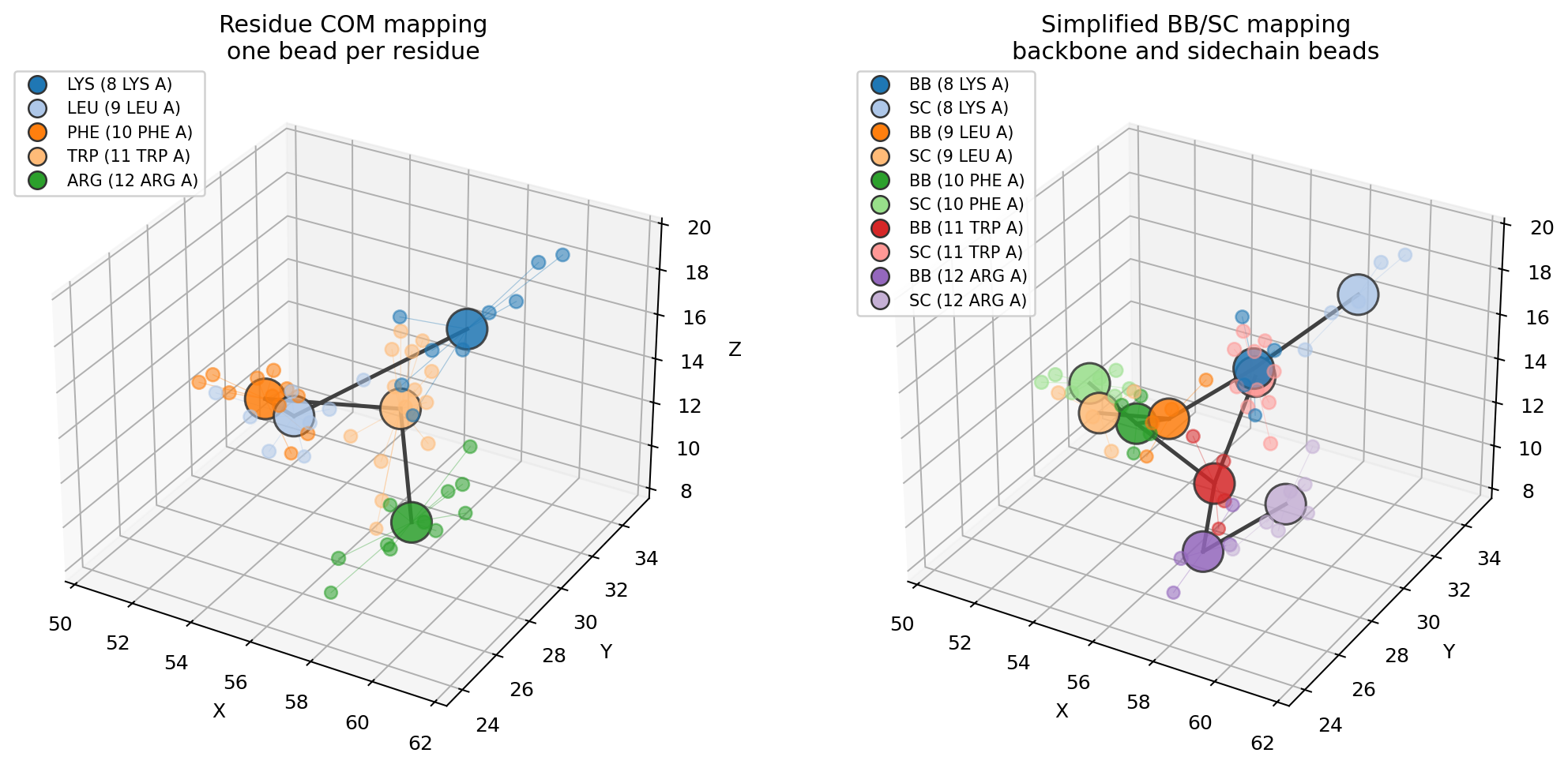
plot_mapping overlays the beads on the atoms they replace, colouring each atom by its bead. A short fragment reads most clearly:

fragment = mol.select(resid=(8, 12))
ms.plot_mapping(fragment, fragment.coarse_grain("martini"))

For a side-by-side residue COM vs backbone/sidechain visual:

uv run python examples/coarse_graining.py

Inspect and export the assignment

report = cg.coarse_grain_report
print(report.coverage())              # beads / atoms covered
print(report.beads[0].atom_indices)    # which atoms became bead 0

cg.write_mapping("mapping.json")      # JSON record (round-trippable)
cg.write_index("mapping.ndx")         # GROMACS-style index, one group per bead

record = ms.read_cg_mapping("mapping.json")
cg_again = ms.apply_cg_mapping(mol, record)   # rebuild on the same structure