PDB to Coarse-Grained Beads

This tutorial maps an atomistic PDB structure to lower-resolution beads. The goal is inspection, teaching, and graph prototyping: MolScope does not generate production Martini topology files or force-field parameters.

You will build:

• one bead per residue using a center-of-mass mapping,
• a backbone/sidechain bead model inspired by Martini-style mappings,
• a mapping report plus JSON and index exports.

Read a protein and choose a fragment

The full 1fqy.pdb structure is useful for counts. A short residue slice is easier to visualize:

import molscope as ms

mol = ms.read("examples/data/1fqy.pdb")
fragment = mol.select(resid=(8, 12))

print(len(mol), "atomistic atoms")
print(len(list(mol.residue_groups())), "residues")
print(len(fragment), "atoms in the tutorial fragment")

For the bundled data, the fragment contains 53 atoms across 5 residues.

One bead per residue

cg = fragment.coarse_grain("residue_com")

print(len(cg), "beads")
print(len(cg.bonds()), "CG bonds")
print(cg.coarse_grain_report.coverage())

Expected output:

5 beads
4 CG bonds
5 beads from 53/53 atoms

residue_com places each bead at the mass-weighted center of all atoms in that residue. Use residue_centroid when you want the unweighted geometric center instead:

centroid_cg = fragment.coarse_grain("residue_centroid")

Backbone and sidechain beads

The simplified martini mapping splits each residue into a backbone bead and, when sidechain heavy atoms exist, a sidechain bead:

bb_sc = fragment.coarse_grain("martini")

print(len(bb_sc), "beads")
print(len(bb_sc.bonds()), "CG bonds")
print(bb_sc.atom_names[:6])

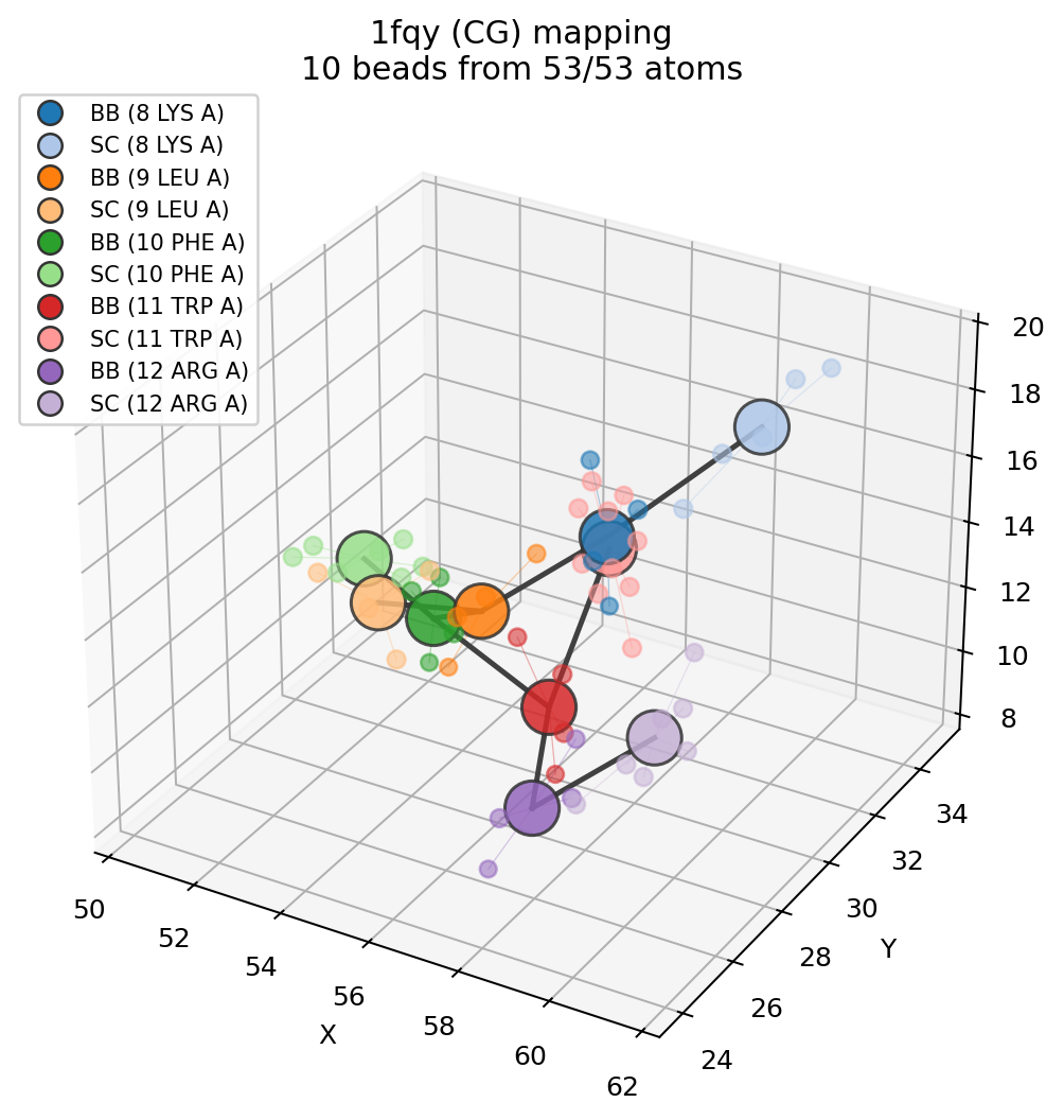
For the same 5-residue fragment, this produces 10 beads and 9 simple CG bonds. The bead names are intentionally familiar (BB, SC) but this is not a complete Martini model: real production models also need bead types, charges, bonded terms, nonbonded parameters, exclusions, and validation.

Add an explicit virtual site

Some Martini/GROMACS workflows use virtual sites: coordinates derived from other particles rather than ordinary integrated beads. MolScope supports that mapping metadata explicitly for inspection and graph prototyping:

bb_sc_vs = fragment.coarse_grain(
    "martini",
    virtual_sites=[{"name": "MID", "parents": [0, 2]}],
)

site = bb_sc_vs.coarse_grain_report.virtual_sites[0]
print(site.name, site.parents, site.rule, site.weights)
print(bb_sc_vs.virtual_sites.tolist())

The virtual site is appended after the real beads and marked in bb_sc_vs.virtual_sites. Parent references are bead indices in the CG model before virtual sites are appended. For repeated bead names such as BB and SC, use indices rather than names.

Virtual sites are preserved in mapping JSON and graph exports, but MolScope does not write production GROMACS [ virtual_sites* ] topology sections.

Visualize the atom-to-bead mapping

ms.plot_mapping(fragment, bb_sc)

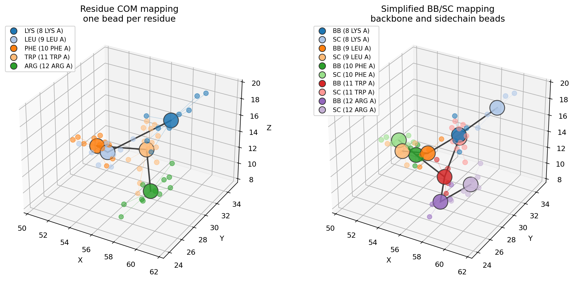
The mapping plot draws atomistic atoms, translucent beads, assignment lines, and the CG bond network.

For a side-by-side comparison of residue-center and backbone/sidechain representations, run:

uv run python examples/coarse_graining.py

Inspect the mapping report

Every CG molecule keeps a structured report describing which source atoms were assigned to each bead:

report = bb_sc.coarse_grain_report

print(report.coverage())
print(report.n_beads, report.n_assigned, report.n_dropped)

first = report.beads[0]
print(first.name, first.resname, first.resid, first.chain)
print(first.atom_indices)
print(first.atom_names)

For a readable text report:

print(bb_sc.mapping_report())

This is the first place to look when a custom mapping drops atoms or creates a different bead count than expected.

Export the mapping

Write the bead assignment to JSON for round-tripping:

bb_sc.write_mapping("fragment_mapping.json")

record = ms.read_cg_mapping("fragment_mapping.json")
rebuilt = ms.apply_cg_mapping(fragment, record)

Write a GROMACS-style index file for inspection in tools that understand .ndx groups:

bb_sc.write_index("fragment_mapping.ndx")

The bead model itself is still a Molecule, so ordinary coordinate export also works:

ms.write_pdb(bb_sc, "fragment_beads.pdb")

The PDB contains bead coordinates and CONECT records for the CG bond network. It is useful for inspection and graph workflows, not for production simulation.

Custom mappings

For teaching or domain-specific prototypes, define the atoms that belong to each bead:

mapping = {
    "ALA": {
        "BB": ["N", "CA", "C", "O"],
        "SC": ["CB"],
    }
}

custom = fragment.coarse_grain(mapping)
print(custom.mapping_report())

Name-based custom bonds work best when bead names are unique. If repeated names such as BB and SC appear across residues, use bead indices for explicit bond definitions.

Scale up to the full structure

full_residue_cg = mol.coarse_grain("residue_com")
full_martini_like = mol.coarse_grain("martini")

print(len(full_residue_cg), "residue beads")
print(len(full_martini_like), "backbone/sidechain beads")

Use the full model for graph export, residue-level comparisons, or quick structure summaries. Use small fragments when you need to visually inspect the mapping.